Don’t worry about high SWR!

One often hears hams saying that they are concerned that they cannot get their SWR down to 1:1. Actually, if things are done right, an SWR of 3:1, or even higher, isn’t a problem. This leads to a lot of possibilities which are discussed in this article:

Why a properly designed antenna system will radiate the entire transmitter’s power with very little loss regardless of the antenna system’s SWR.
How to build a simple dipole that will work on all ham bands and even provide gain on the higher ham bands.

There are two issues for getting all the transmitter power radiated: getting all the power into the transmission line and then getting the antenna to radiate it.

Getting All Power into a Transmission Line Having High SWR

Two block diagrams. In (a) a 100 watt source feeds a 50 ohm line into a 16 ohm load and 25 watts is reflected back into the transmitter, so only 75 watts goes down the line. In (b) a tuner sits between them, presenting 100 minus j240 ohms to the line and 100 plus j240 ohms to the source, and all 100 watts is delivered. — **Figure 1.** Getting all the power into the transmission line. Without a match at the source (a), power is reflected back into the transmitter; with a conjugate match (b), all of it goes down the line.
Drawing: Bill Rinker, W6OAV

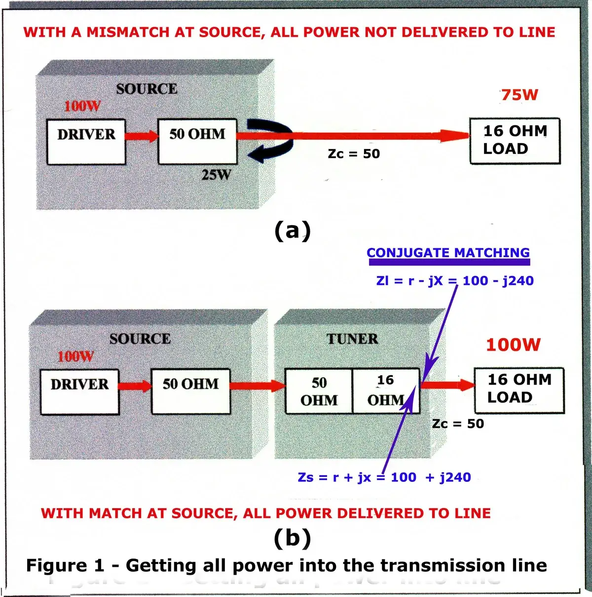
Figure 1(a) shows that all the transmitted power is not delivered to a transmission line when there is a mismatch between the transmitter’s output impedance and the transmission line’s input impedance. In this example, 25 percent of the power is reflected back into the transmitter and heating up the transmitter’s final amplifiers. So, how do we get all the power from the transmitter into the transmission line? We use a good tuner. The tuner uses conjugate matching to deliver all the power into the transmission line. Conjugate matching means that if a load has a certain resistance and a certain reactance, the source will have that same resistance and equal but opposite reactance. Figure 1(b) shows conjugate matching. The transmission line has an input impedance which has an inductive reactance (-j240) and a resistance of 100 ohms. The tuner, when tuned for maximum power transfer to the transmission line, has an equal but opposite capacitive reactance (+j240) and an equal resistance of 100 ohms.

What happens now that all power is in the transmission line?

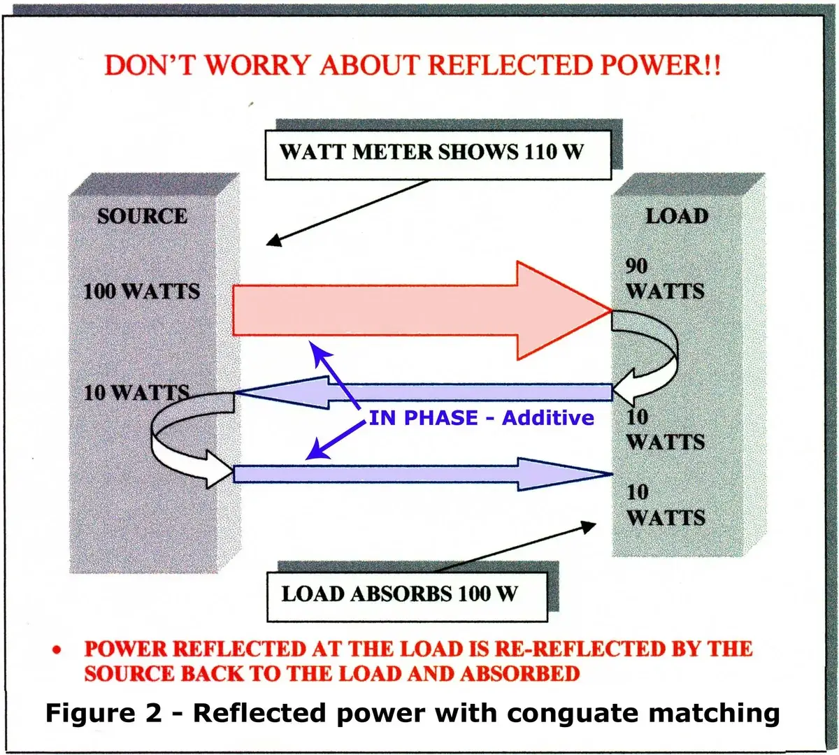
The following discussion uses a perfect 0 dB loss transmission line. Later, we’ll discuss a real world transmission line having some loss. So, now that we have all the transmitter power going into the transmission line, what happens at the mismatch between the transmission line and the antenna? Some of the power is reflected back to the tuner. However, this power is not lost. When the reflected power arrives at the tuner, due to the properties of the tuner’s conjugate match, the power is re-reflected in phase with the transmitted power back to the antenna.

Diagram showing 100 watts leaving the source, 90 watts absorbed by the load and 10 watts reflected back, where the source re-reflects it in phase so it returns to the load and is absorbed. The watt meter reads 110 watts while the load still absorbs 100 watts. — **Figure 2.** Reflected power with a conjugate match. Power reflected at the load is re-reflected by the source, in phase, and ends up in the antenna after all.
Drawing: Bill Rinker, W6OAV

Figure 2 shows an example where, due to the mismatch between the transmission line and the antenna, 10 percent of the power is reflected back at the antenna. However, that power is re-reflected at the tuner in phase with the transmitter power where it is absorbed by the antenna. In other words, all power delivered to the transmission line will be absorbed by the antenna, no matter what the SWR. Depending upon the degree of mismatch, there may be another smaller third reflection from the antenna back to the tuner where it is re-reflected in phase with the transmitter power back to the antenna. For those interested in the math and the explanations behind this action, refer to the references below.

Now, let’s discuss the real world with coax loss. In this example, we’ll use 100 ft of RG-213 coax to illustrate how the loss of coax affects the amount of power delivered to, and radiated by, an antenna at various SWR values. 100 ft of RG-213 with an SWR of 1:1 has 0.642 dB loss at 28 MHz. (We’re using 28 MHz as the coax has more loss at that frequency compared to lower frequencies.) Let’s look at what happens when this coax is used with an antenna producing an SWR of 3:1.

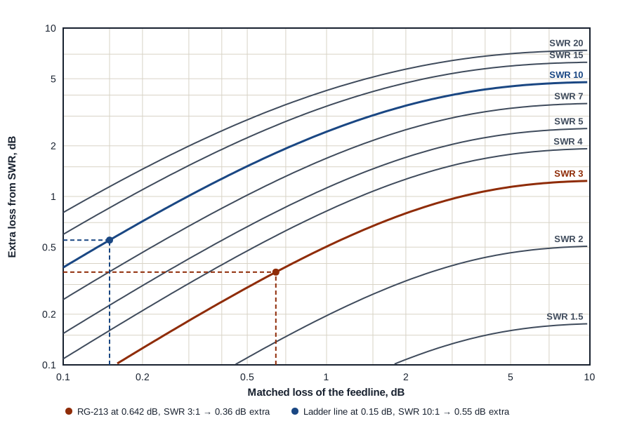
Log-log chart. The horizontal axis is the matched loss of a feedline in decibels, from 0.1 to 10. The vertical axis is the extra loss caused by standing waves, also 0.1 to 10 decibels. One curve per SWR value from 1.5 to 20 rises to the right. Markers show 100 feet of RG-213 at 28 megahertz, 0.642 dB matched, gaining 0.36 dB extra at an SWR of 3 to 1, and 100 feet of ladder line at 0.15 dB matched, gaining 0.55 dB extra at an SWR of 10 to 1. — **Figure 3.** How much extra loss standing waves really cost. Start at the feedline’s matched loss along the bottom, go up to the SWR curve, and read the extra loss on the left. *Drawn for OneShack from the standard transmission-line equations*

Figure 3 shows the extra loss of a feedline at various values of SWR. For example, to determine what happens to power loss when the SWR increases from 1:1 to 3:1, draw a vertical line on the horizontal axis from the 0.642 dB point (RG-213 loss at 28 MHz with an SWR of 1:1) up to the SWR 3 curve. Then draw a horizontal line from the SWR 3 curve to the left vertical axis. This shows that the additional loss caused by an SWR of 3:1 is only 0.356 dB. Thus the total transmission loss went from 0.642 dB to 0.998 dB. Table 1 summarizes these results.

Power into the line	Matched loss	Extra loss from SWR	Total loss	Power out
100 W	SWR 1:1 — 0.642 dB	0.0 dB	0.642 dB	86.26 W
100 W	SWR 3:1 — 0.642 dB	0.356 dB	0.998 dB	79.48 W

Table 1. 100 ft of RG-213 at 28 MHz.

There are many good SWR versus extra loss calculators available, including the one on this site. These calculators allow experimenting with different types of feed lines to see what happens as the SWR increases.

The above discussion illustrates that if a high quality transmission line and a good tuner are used, high SWRs will not cause a noticeable additional transmitted power loss. This does not mean that you should ignore high SWR. You should have a reasonable idea of what SWR is expected. For example, if a dipole cut to resonance has an SWR of 3:1, then there is a problem. A typical dipole in the clear should range between 1.2:1 and 1.8:1 depending upon the dipole’s height above ground. Also, use caution when running a fair amount of power with systems having a high SWR. Coax losses result in power being dissipated inside the coax and higher voltages between the center conductor and the outer shield. This can cause a nasty flash over within the coax.

Building a Simple All Band Lossless Dipole

So, based on the above discussion, how do we design an all band dipole that has virtually no extra loss at high values of SWR and no high voltage flash over issues? We use open wire feed line or ladder line. Looking again at Figure 3, the extra loss of ladder line caused by various SWRs is so small that the losses barely register: the matched loss of ladder line at 28 MHz is only about 0.15 dB, and even with an SWR of 10:1 the extra loss is only 0.551 dB. Table 2 summarizes the losses.

Power into the line	Matched loss	Extra loss from SWR	Total loss	Power out
100 W	SWR 1:1 — 0.15 dB	0.0 dB	0.15 dB	96.60 W
100 W	SWR 10:1 — 0.15 dB	0.551 dB	0.702 dB	85.08 W

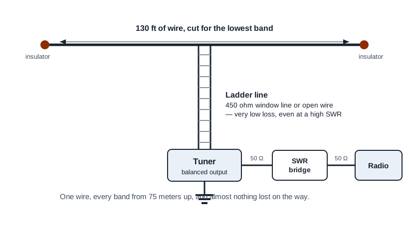
Table 2. 100 ft of ladder line at 28 MHz.

Based on the above discussion, how do we build an all band dipole which has virtually no loss at the lowest band of interest and gain at the upper bands? We build a half wave dipole cut for the lowest band of interest and feed it with open wire or ladder line as shown in Figure 4.

Drawing of an all-band dipole: a 130-foot wire dipole fed at its center with ladder line running down to an antenna tuner, which connects through an SWR bridge to the transmitter. — **Figure 4.** The all-band dipole: one wire cut for the lowest band, fed with ladder line into a tuner. *Drawn for OneShack*

For example, EZNEC antenna analysis shows that a 75 meter dipole 45 ft above ground and fed with ladder line will show the gains listed in Table 3. The gain results because, as the frequencies increase from 3.65 MHz to 28.3 MHz, the pattern changes from a broad figure 8 to a narrower four leaf clover, thus concentrating the power in narrower lobes.

Frequency (MHz)	Gain (dBi)
3.65	6.87
7.10	7.24
10.14	8.66
14.18	6.56
18.11	7.76
21.25	10.93
24.90	10.65
28.30	10.52

Table 3. A 75 meter dipole 45 ft up, fed with ladder line: gain by band.

From an EZNEC analysis. The gain figures are at the peak of the horizontal pattern; as the frequency rises that peak moves lower in elevation.

Depending upon the height of the antenna and the length of feed line, the tuner might not be able to match the antenna on a particular band.

Summary

The cardinal rule is that if a high quality transmission line and a good tuner are used, high SWRs will not cause a noticeable transmitted power loss. This rule also allows the ability to use a single efficient dipole on many different bands.

References

OneShack: Coax Loss & dB calculator